


Previously on…
In the first post of this series, we implemented a simple binary classifier. In this post, we will adapt it to a softmax classifier.
Softmax
The binary classifier’s output is a single value between 0 and 1. In as such it can only be used to classify between two classes. The softmax classifier, on the other hand, can be used to classify between multiple classes.
In the previous post we took a dataset of the images of bean plants and classified them as either healthy or diseased. However the original dataset contains 3 labels: ‘angular_leaf_spot’, ‘bean_rust’, and ‘healthy’.
Let’s change the Neural Network we built the last time to be able to classify between these 3 classes.
The output layer
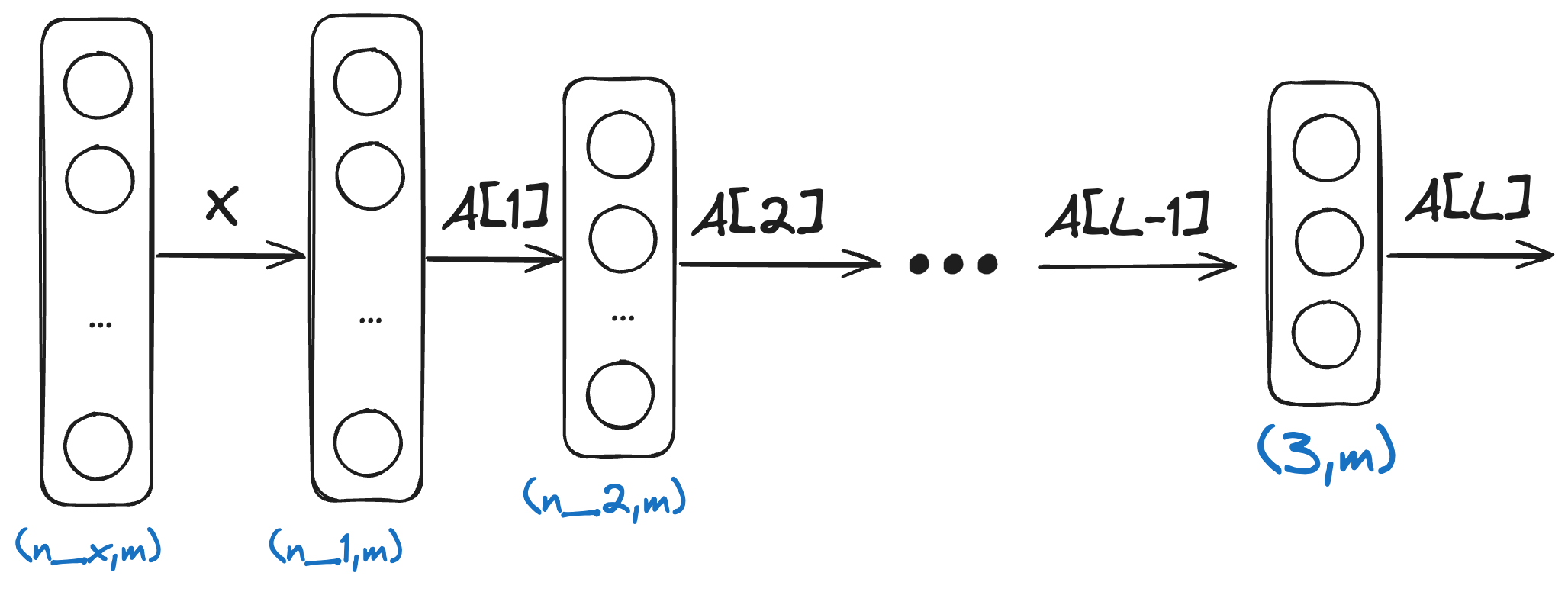
The output layer of the softmax classifier will have 3 neurons, one for each class. The output of the network will be a vector of 3 values between 0 and 1, each value representing the probability of the input image belonging to the corresponding class.
Adapting the network
The way we initialise weights and biases and run forward propagation stays exactly the same as with the binary classifier:
1
2
3
4
5
6
7
8
9
10
11
12
13
14
15
16
17
18
19
20
21
22
23
24
25
26
27
28
29
30
import numpy as np

def initialise_parameters(X, nn_shape):
    parameters = {}

    # Number of features in an example
    n_x = X.shape[0]

    for i, layer in enumerate(nn_shape):
        n_prev = n_x if i == 0 else nn_shape[i-1]["nodes"]
        parameters[f"W{i+1}"] = np.random.randn(layer["nodes"], n_prev) * np.sqrt(2. / n_prev)
        parameters[f"b{i+1}"] = np.zeros((layer["nodes"], 1))

    return parameters

def forward_prop(X, params, nn_shape):
    grads = {"A0": X}

    for l, layer in enumerate(nn_shape):
        W = params[f"W{l+1}"]
        b = params[f"b{l+1}"]
        A_prev = grads[f"A{l}"]

        Z = np.dot(W, A_prev) + b
        A = activations[layer["activation"]](Z)

        grads[f"Z{l+1}"] = Z
        grads[f"A{l+1}"] = A

    return grads
The hidden layers will still use the ReLU activation function:
1
2
3
4
def relu(Z):
    A = np.maximum(0,Z)

    return A
Softmax activation function
The softmax activation function is computed as follows:
\[\sigma(z)_j = \frac{e^{z_j}}{\sum_{k=1}^{K} e^{z_k}}\]Where \(z\) is the output of the last layer of the network, and \(K\) is the number of classes.
Let’s implement it:
1
2
3
4
def softmax(Z):
    exsps = np.exp(Z)
    A = exsps / np.sum(exsps, axis=0, keepdims=True)
    return A
Loss function
The loss function for the softmax classifier is the cross-entropy loss:
\[L(y, \hat{y}) = -\sum_{i=1}^{K} y_i \log(\hat{y}_i)\]Where \(y\) is the true label of the input, and \(\hat{y}\) is the output of the network.
Note that \(Y\) is the original vector of labels:
One-hot encoding
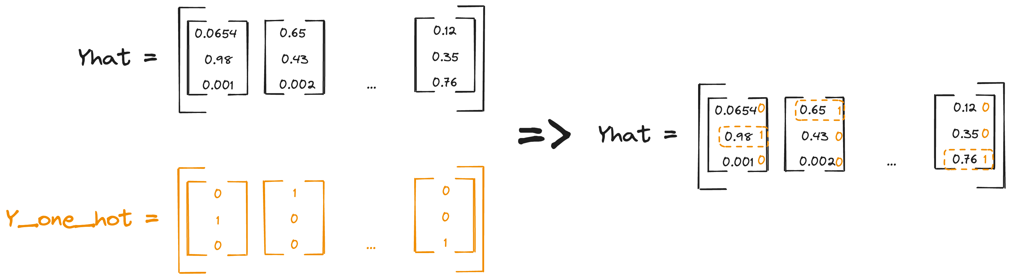
A “one-hot encoded” vector of the labels is a matrix where each example is a vector of 0s and a single 1 at the index of the true label. E.g. if \(Y = [0,1,2]\), the one-hot encoded matrix is:
\[Y = \begin{bmatrix} 1 & 0 & 0 \\ 0 & 1 & 0 \\ 0 & 0 & 1 \end{bmatrix}\]Implementing the cost function
The output of the softmax classifier is a matrix \((K,m)\), where \(m\) is the number of examples and \(K\) is the number of classes.
To compute the loss we essentially need to sum the logarithms of every value in the output that corresponds to the “correct label”. To do this with numpy we can employ a neat trick: we can use the one-hot encoded matrix to index the output matrix.
1
Yhat[Y,range(m)]
The cost function therefore can be computed as:
1
2
3
def compute_cost_softmax(Y, Yhat):
    m = Y.shape[0]
    return np.sum(-np.log(Yhat[Y,range(m)] + 1e-9)) / m
We add a small constant 1e-9 to the logarithm to avoid numerical instability in cases where the predicted value is close to 0, as the logarithm of 0 is undefined.
Adapting the backpropagation
In the previous post we defined the backpropagation functions for a binary classifier as follows:
1
2
3
4
5
6
7
8
9
10
11
12
13
14
15
16
17
18
19
20
21
22
23
24
25
26
27
28
29
30
31
32
33
34
35
36
37
38
39
def back_prop(X, Y, params, grads, nn_shape, learning_rate=0.001):
    # Number of examples
    m = Y.shape[0]
    # Number of layers
    L = len(nn_shape)

    # Iterate over the layers, last to first
    for l in range(L, 0, -1):
        W = params[f"W{l}"]
        b = params[f"b{l}"]
        Z = grads[f"Z{l}"]
        A = grads[f"A{l}"]

        # Compute dZ[l] for the last layer with the sigmoid activation function
        if nn_shape[l-1]["activation"] == "sigmoid":
            dZ = A - Y

        # Compute dZ[l] for the hidden layers
        if nn_shape[l-1]["activation"] == "relu":
            dZnext = grads[f"dZ{l+1}"]
            Wnext = params[f"W{l+1}"]
            dA = np.dot(Wnext.T, dZnext)
            grads[f"dA{l}"] = dA

            dZ = np.array(dA, copy=True)
            dZ[Z < 0] = 0

        Aprev = X if l == 1 else grads[f"A{l-1}"]
        dW = (1/m) * np.dot(dZ, Aprev.T)
        db = (1/m) * np.sum(dZ, axis=1, keepdims=True)

        W = W - learning_rate * dW
        b = b - learning_rate * db

        params[f"W{l}"] = W
        params[f"b{l}"] = b
        grads[f"dZ{l}"] = dZ

    return params
The only thing we need to change is to compute dZ for the softmax layer, which is calculated as follows:
1
dZ = A - Y_one_hot
Where A is the activation of the last layer. So the new back_prop function becomes:
1
2
3
4
5
6
7
8
9
10
11
12
13
14
15
16
17
18
19
20
21
22
23
24
25
26
27
28
29
30
31
32
33
34
35
36
def back_prop(X, Y, Y_one_hot, params, grads, nn_shape, learning_rate=0.001):
    L = len(nn_shape)
    m = Y.shape[0]

    for l in range(L, 0, -1):
        W = params[f"W{l}"]
        b = params[f"b{l}"]
        A = grads[f"A{l}"]
        Z = grads[f"Z{l}"]

        if nn_shape[l-1]["activation"] == "sigmoid":
            dZ = A - Y
        if nn_shape[l-1]["activation"] == "softmax":
            dZ = A - Y_one_hot
        if nn_shape[l-1]["activation"] == "relu":
            dZnext = grads[f"dZ{l+1}"]
            Wnext = params[f"W{l+1}"]
            dA = np.dot(Wnext.T, dZnext)
            grads[f"dA{l}"] = dA

            dZ = np.array(dA, copy=True)
            dZ[Z < 0] = 0

        Aprev = X if l == 1 else grads[f"A{l-1}"]
        dW = (1/m) * np.dot(dZ, Aprev.T)
        db = (1/m) * np.sum(dZ, axis=1, keepdims=True)

        W = W - learning_rate * dW
        b = b - learning_rate * db

        grads[f"dZ{l}"] = dZ
        params[f"W{l}"] = W
        params[f"b{l}"] = b


    return params
Putting it all together
Let’s define a train function and train the network on the bean dataset:
1
2
3
4
5
6
7
8
9
10
11
12
13
14
15
16
17
18
19
20
21
22
23
24
25
26
27
28
29
30
31
32
33
34
35
36
37
38
39
40
41
# In the helper module

def train(X, Y, nn_shape, epochs=1000, learning_rate=0.001):
    L_activation = nn_shape[-1]["activation"]
    params = initialise_parameters(X, nn_shape)
    m = Y.shape[0]
    Y_one_hot = np.zeros((3, m)) # 3 is the number of classes
    Y_one_hot[Y, np.arange(Y.size)] = 1
    for epoch in range(epochs):
        grads = forward_prop(X, params, nn_shape)
        if L_activation == "softmax":
            cost = compute_cost_softmax(Y, grads[f"A{len(nn_shape)}"])
        else:
            cost = compute_cost_binary(Y, grads[f"A{len(nn_shape)}"])
        params = back_prop(X, Y, Y_one_hot, params, grads, nn_shape, learning_rate)
        if epoch % 100 == 0:
            print(f"Cost after epoch {epoch}: {cost}")
    return params

#----------------------------------------------

# In the Jupyter notebook

from image_classifier import predict, accuracy, train
import image_classifier as nn

# importlib.reload(nn) will reload the imported module every time you run the cell.
# This is handy for making changes to the module and testing them without restarting the kernel.
import importlib
importlib.reload(nn)

# Beefing up the network a little bit compared to the binary classifier to increase accuracy
nn_shape_softmax = [
    {"nodes": 10, "activation": "relu"},
    {"nodes": 10, "activation": "relu"},
    {"nodes": 10, "activation": "relu"},
    {"nodes": 3, "activation": "softmax"},
]
print("X_train: ", X_train.shape)
print("Y_train: ", Y_train.shape)
params = nn.train(X_train, Y_train, nn_shape_softmax, 1000, 0.001)
Output:
Y_train: (1034,)
Cost after epoch 0: 1.1173747027140468
Cost after epoch 100: 0.9726746857697608
Cost after epoch 200: 0.928352099068845
Cost after epoch 300: 0.9064075741942758
Cost after epoch 400: 0.876434678998784
Cost after epoch 500: 0.8295728893517074
Cost after epoch 600: 0.8062364047067908
Cost after epoch 700: 0.8309177076189542
Cost after epoch 800: 0.7651304635068248
Cost after epoch 900: 0.7717121220077787
Measuring accuracy the same way as for the binary classifier, we get these numbers:
Accuracy on the dev set: 0.5939849624060151
Which is not great, especially on the dev set. In the next post we will experiment with different optimisation tactics.